Tutorial

We will first test that MDAnalysis can perform PSA, using the small test set. We will then look in detail into the radical.pilot script that implements the map-step. Finally, we conclude with the reduce-step and analysis of the data.

Preliminary test

Provide topology and trajectory files to the PSA script mdanalysis_psa_partial.py as two lists in a JSON file (see mdanalysis_psa_partial.py for more details). Initially we just want to check that the script can process the data

(mdaenv) $ $RPDIR/mdanalysis_psa_partial.py --inputfile testcase.json -n 5

This means

• use the test case

• compare the first 5 trajectories against the remaining 5 trajectories

The -n (split) argument is important because we are going to use it to decompose the full distance matrix into sub-matrices. (If you just want to do all-vs-all comparisons, use the mdanalysis_psa.py script.)

You should see output like

Loading paths from JSON file testcase.json
Processing 10 trajectories.
Splitting trajectories in two blocks of length 5 and 5
Calculating D (shape 5 x 5) with 25 entries
----------[ TIMING ]--------------------
load Universes                     0.448 s
universe.transfer_to_memory()      0.178 s
PSA distance matrix                1.483 s
saving output                      0.001 s
----------------------------------------
total time                         2.111 s
----------------------------------------

This indicates that all MDAnalysis parts are working.

Similarly:

(mdaenv) $ $RPDIR/mdanalysis_psa_partial.py --inputfile testcase.json -n 7

should give something like

Loading paths from JSON file testcase.json
Processing 10 trajectories.
Splitting trajectories in two blocks of length 7 and 3
Calculating D (shape 7 x 3) with 21 entries
----------[ TIMING ]--------------------
load Universes                     0.422 s
universe.transfer_to_memory()      0.132 s
PSA distance matrix                1.436 s
saving output                      0.001 s
----------------------------------------
total time                         1.991 s
----------------------------------------

Supercomputer environment

We used TACC Stampede to run the calculations on 32 cores but any cluster or even a multi core workstation might be sufficient.

• Make sure all env vars are set (especially MongoDB, RADICAL_PILOT_DBURL) and password-less ssh works.

• On stampede: Set environment variable RADICAL_PILOT_PROJECT to your XSEDE allocation:

  export RADICAL_PILOT_PROJECT=TG-xxxxxx
  

• Activate the mdaenv environment.

• You should have the JSON files in the WORK directory.

Copy the two scripts to the WORK directory (at the moment, this is a limitation of the scripts to keep them simple)L

cd WORK
cp $RPDIR/{rp_psa.py,mdanalysis_psa_partial.py} .

Map-step: Radical.pilot script

RP script

The pilot script is rp/rp_psa.py (see rp_psa.py for details). In the following, important parts of the script are explained.

First, a session is created and a Pilot Manager is initialized:

        session   = rp.Session (name=session_name)
        c         = rp.Context ('ssh')
        session.add_context (c)

        print "initialize pilot manager ..."
        pmgr = rp.PilotManager (session=session)

Second, a ComputePilot is described and submitted to the Pilot Manager:

        pdesc = rp.ComputePilotDescription ()
        pdesc.resource = "xsede.stampede"   # xsede.stampede or xsede.comet or ... check docs!
        pdesc.runtime  = 20 # minutes
        pdesc.cores    = cores
        pdesc.project  = PROJECT #Project allocation, pass through env var PROJECT
        pdesc.cleanup  = False
        pdesc.access_schema = 'ssh'

        # submit the pilot.
        pilot = pmgr.submit_pilots (pdesc)

First, a Unit Manager is created for that session and the Pilot is added:

        umgr = rp.UnitManager  (session=session, scheduler=rp.SCHED_DIRECT_SUBMISSION)

        #add pilot to unit manager
        umgr.add_pilots(pilot)

The script reads the topology and trajectory files from a JSON file:

        with open(FILELIST) as inp:
            topologies, trajectories = json.load(inp)

The MDAnalysis script is staged

        fname_stage = []
        # stage all files to the staging area
        src_url = 'file://%s/%s' % (os.getcwd(), SHARED_MDA_SCRIPT)

        #print src_url

        sd_pilot = {'source': src_url,
                    'target': os.path.join(MY_STAGING_AREA, SHARED_MDA_SCRIPT),
                    'action': rp.TRANSFER,
        }
        fname_stage.append(sd_pilot)

        # Synchronously stage the data to the pilot
        pilot.stage_in(fname_stage)

In a loop, a CU is set up for each block matrix — this is the map step. In particular, the trajectories are partitioned according to the BLOCK_SIZE (the parameter \(w\)) and all necessary information is written to a JSON file that will be used as the input for the mdanalysis_psa_partial.py script:

        cudesc_list = []

        for i in range(0, len(trajectories), BLOCK_SIZE):
            for j in range(i, len(trajectories), BLOCK_SIZE):
                fshared = list()
                shared = {'source': os.path.join(MY_STAGING_AREA, SHARED_MDA_SCRIPT),
                          'target': SHARED_MDA_SCRIPT,
                          'action': rp.LINK}
                fshared.append(shared)

                shared = [{'source': 'file://{0}'.format(trajectory),
                           'target' : basename(trajectory),
                           'action' : rp.LINK}
                              for trajectory in trajectories[i:i+BLOCK_SIZE]]
                fshared.extend(shared)
                if i!=j:
                    shared = [{'source': 'file://{0}'.format(trajectory),
                               'target' : basename(trajectory),
                               'action' : rp.LINK}
                                  for trajectory in trajectories[j:j+BLOCK_SIZE]]
                    fshared.extend(shared)
                # always copy all unique topology files
                shared = [{'source': 'file://{0}'.format(topology),
                           'target' : basename(topology),
                           'action' : rp.LINK}
                          for topology in set(topologies)]
                fshared.extend(shared)

                # block of topology / trajectory pairs
                #   block[:nsplit] + block[nsplit:]
                # The MDA script wants one long list of trajectories and the index nsplit
                # that indicates where to split the list to create the two groups of
                # trajectories that are compared against each other.
                block_top = topologies[i:i+BLOCK_SIZE] + topologies[j:j+BLOCK_SIZE]
                block_trj = trajectories[i:i+BLOCK_SIZE] + trajectories[j:j+BLOCK_SIZE]
                block = [block_top, block_trj]
                nsplit = len(trajectories[i:i+BLOCK_SIZE])
                imax = i + len(trajectories[i:i+BLOCK_SIZE])
                jmax = j + len(trajectories[j:j+BLOCK_SIZE])
                # should remember i, imax and j_jmax because we calculate the
                # submatrix D[i:i+di, j:j+dj] in this CU.
                block_json = "block-{0}-{1}__{2}-{3}.json".format(
                    i, imax, j, jmax)
                block_matrixfile = 'subdistances_{0}-{1}__{2}-{3}.npy'.format(
                    i, imax, j, jmax)

                manifest.append((block_matrixfile, block_json, (i, imax), (j, jmax)))

                # create input file for the cu and add share it
                with open(block_json, "w") as out:
                    json.dump(block, out)

                # share input json file
                shared = [{'source': 'file://{0}'.format(os.path.realpath(block_json)),
                           'target' : basename(block_json),
                           'action' : rp.LINK}
                ]
                fshared.extend(shared)

                # define the compute unit, to compute over the trajectory submatrix
                # TODO: store the offsets WITH the returned matrix (pkl or arrach archive) instead
                #       of encoding in filename
                cudesc = rp.ComputeUnitDescription()
                cudesc.executable     = "python"
                cudesc.pre_exec       = ["module load python; source activate mdaenv"] #Only for Stampede and with our conda env
                cudesc.input_staging  = fshared
                cudesc.output_staging = {'source': block_matrixfile,
                                         'target': block_matrixfile,
                                         'action': rp.TRANSFER}
                cudesc.arguments      = [SHARED_MDA_SCRIPT, '--nsplit', nsplit,
                                         '--inputfile', block_json,
                                         '--outfile', block_matrixfile, ]
                cudesc.cores          = 1

                cudesc_list.append(cudesc)

For the reduce step, all information about the block matrix (filename and indices in the distance matrix) are written to a JSON file (“manifest”):

        with open(MANIFEST_NAME, "w") as outfile:
            json.dump(manifest, outfile)

Finally, the CUs are submitted to execute on the compute resources and the script waits until they are all complete:

        # submit, run and wait and...
        #print "submit units to unit manager ..."
        units = umgr.submit_units(cudesc_list)

        #print "wait for units ..."
        umgr.wait_units()

Launch pilot jobs

Launch the pilot job from the login node of stampede (or the cluster where you set up your radical.pilot environment):

python rp_psa.py trajectories.json 20 16 SPIDAL.001

The rp_psa.py radical.pilot script takes as input (see rp_psa.py for details):

• the JSON file with the trajectories (trajectories.json)

• number of trajectories per block (20)

• number of cores to request (16)

• session name (arbitrary string, “SPIDAL.001”); note that you need to provide a new session name every time you-rerun the command, e.g. “SPIDAL.002”, “SPIDAL.003”, …

Reduce-step

Once the pilot jobs has completed and all block matrices have been computed we combine all data (reduce) into the distance matrix \(D_{ij}\) and analyze it:

psa_reduce.py -t trajectories.json -m manifest.json \
              -p psa_plot.pdf -o distance_matrix.npy

Combine block matrices

The manifest.json file contains all information that is needed to re-assemble the distance matrix: for each output file it also stores the indices of the sub-matrix in the distance matrix and so the full distance matrix can be built with

def combine(traj, manifest):
    trj = json.load(open(traj))
    N = len(trj[0])
    D = np.zeros((N, N))

    mf = json.load(open(manifest))

    missing = []
    for subD, _, (i0, i1), (j0, j1) in mf:
        try:
            D[i0:i1, j0:j1] = np.load(subD)
            D[j0:j1, i0:i1] = D[i0:i1, j0:j1].T
        except IOError:
            missing.append(subD)

    if missing:
        print("WARNING: Missing data: output files\n{}\n"
              "could not be found".format(", ".join(missing)))

    return D

The matrix is written to a numpy file distance_matrix.npy (and can be loaded with numpy.load()).

Analysis

The distance matrix can be clustered to reveal patterns in the trajectories. Here we use hierarchical clustering with Ward’s linkage criterion as implemented in scipy.cluster.hierarchy [Seyler2015]. The clustering and plotting code was taken from the cluster() and plot() methods of PSAnalysis. The plotting code is fairly complicated but the clustering is straightforward:

def cluster(distArray, method='ward', count_sort=False,
            distance_sort=False, no_plot=False, no_labels=True,
            color_threshold=4):
    """Cluster trajectories and optionally plot the dendrogram.

    :Arguments:
      *method*
        string, name of linkage criterion for clustering [``'ward'``]
      *no_plot*
        boolean, if ``True``, do not render the dendrogram [``False``]
      *no_labels*
        boolean, if ``True`` then do not label dendrogram [``True``]
      *color_threshold*
        For brevity, let t be the color_threshold. Colors all the
        descendent links below a cluster node k the same color if k is
        the first node below the cut threshold t. All links connecting
        nodes with distances greater than or equal to the threshold are
        colored blue. If t is less than or equal to zero, all nodes are
        colored blue. If color_threshold is None or ‘default’,
        corresponding with MATLAB(TM) behavior, the threshold is set to
        0.7*max(Z[:,2]). [``4``]]
    :Returns:
      list of indices representing the row-wise order of the objects
      after clustering
    """
    matplotlib.rcParams['lines.linewidth'] = 0.5

    Z = scipy.cluster.hierarchy.linkage(distArray, method=method)
    dgram = scipy.cluster.hierarchy.dendrogram(
        Z, no_labels=no_labels, orientation='left',
        count_sort=count_sort, distance_sort=distance_sort,
        no_plot=no_plot, color_threshold=color_threshold)
    return Z, dgram

In the resulting plot we indicate FRODA trajectories with a heavy double-bar and DIMS trajectories with a thin single bar.

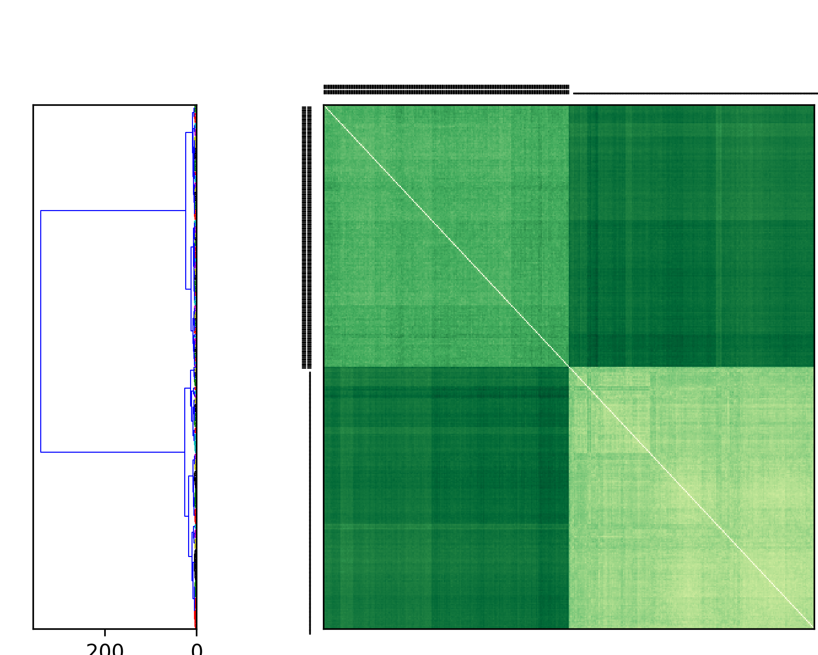
PSA of AdK transitions. Transitions of AdK from the closed to the open conformation were generated with the DIMS MD and the FRODA method. Path similarity analysis (PSA) was performed by hierarchically clustering the matrix of Fréchet distances between all trajectories, using Ward’s linkage criterion.

Symbol	Method
||	FRODA
|	DIMS

Figure PSA of AdK transitions shows clearly that DIMS and FRODA transitions are different from each other. Each method produces transitions that are characteristic of the method itself. In a comparison of many different transition path sampling methods it was also found that this pattern generally holds, which indicates that there is likely no “best” method yet [Seyler2015].