29 Jul 2022
Thanks to the support of a NumFOCUS Small Developer Grant, MDAnalysis is looking to hire a junior developer for 150h (1 month FTE) at 24 USD/hour (3600 USD) to improve the content and organisation of our teaching materials.
MDAnalysis regularly holds workshops to teach researchers how to use our package for their work. We are looking for a junior developer to help us tidy and repackage our teaching materials to provide a cleaner, easier to navigate resource for both users and future workshop creators.
Past workshop materials can be found in the following repos:
Example tasks will include:
- Identifying any outdated material and standardizing contents
- Implementing continuous integration solutions (e.g. nbval) to automatically check and notify if notebook code breaks in the future
- Investigating and implementing new modern notebook extensions to improve the teaching/learning experience
- Identifying any areas where teaching materials are lacking, propose and implement corresponding changes
- Migrating presentation slides to a common, interactive format (e.g., RISE)
- Compiling frequently asked questions in the mailing list in the FAQ page
- Replacing the current outdated MDAnalysis Tutorials page with an overview of all available tutorials, documented and organized by topic/experience level
- Advertising the improvements to the documentation to the MDAcommunity with blog entries and social media posts
You will have the flexibility to decide how to allocate the contract hours, either part-time or full-time, with the commitment to conclude the project by June 2023.
Application requirements
Required criteria
- You have a degree in Chemistry, Chemical Engineering, Physics or a related discipline
- You use molecular dynamics simulations or related techniques in your work
- You use Python, GitHub and Jupyter notebook environments in your work
Desired criteria
- You are familiar with MDAnalysis. Ideally, you already use it or in your research workflows, or have recently attended one of our workshops and now you’re a convert!
- You have contributed code and/or documentation in the computational chemistry/biophysics space. PRs to MDAnalysis repos will be considered a bonus.
Apply by September 1st by filling out this form. Shortlisted candidates will be invited to a zoom interview.
If you have any questions or would like to know more about this opportunity, reach out to Dr Micaela Matta via email using the subject “MDAnalysis junior developer”, or via the MDAnalysis Discord - post in the #jobs channel or DM Micaela(she/her).
19 Jul 2022
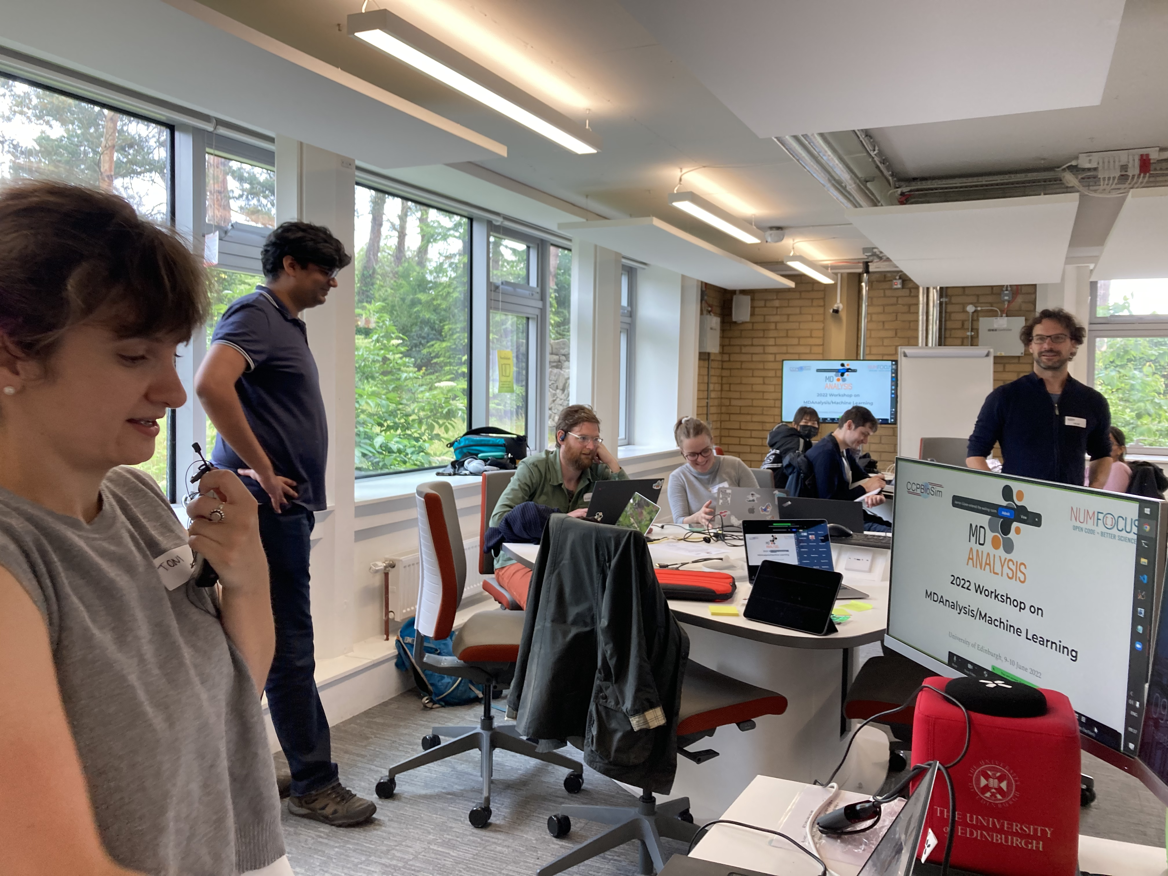
In collaboration with CCPBioSim, 3 MDAnalysis core devs (@ialibay, @micaela-matta, @richardjgowers) together with @ppxasjsm (University of Edinburgh) and @degiacom (University of Durham) organised and ran a 2-day hybrid (in person/online) workshop titled “MDAnalysis and Machine Learning for Molecular Simulations” on June 9-10 2022, immediately following the 8th Annual CCPBioSim Conference.
The workshop received generous funding from the MGMS Early Career Workshop Initiative.
The topics covered included:
- The fundamentals and basics of MDAnalysis
- How to get started with machine learning and tools such as scikit-learn
- How to use MDAnalysis in conjunction with machine learning
- Applying these tools to your own research projects
The workshop was hosted at the University of Edinburgh and consisted of 4 half days in a hybrid format, with over 40 in person attendees and over 30 attendees online at any point in time. A special thank you to Jasmin Güven (PhD student in the group of Antonia Mey) who moderated questions from online participants!
The teaching materials can be run on Google Colab and are found on GitHub.
The workshop style was massively adapted from Software carpentries, using a mixture of life coding, walking through Jupyter notebooks and problem sections. We used the post-it system for instant feedback from participants, and also ran a post-workshop survey, collecting overwhelmingly good feedback.
Thanks to this success, @micaela-matta, @degiacom and @ppxasjsm will be running the workshop again at the CCP5 Summer School on July 26-27 2022, in Durham!
We are glad to see such a high demand for training resources and events from the molecular simulation community. We look forward to continuing to deliver these workshops in the future.
— the MDAnalysis team
17 Jul 2022
MDAnalysis recently attended SciPy 2022!
SciPy was a fantastic opportunity to engage with the open-source
community, build connections and see the amazing work being conducted all
across the Scientific Python ecosystem.
Additionally, Hugo MacDermott-Opeskin presented a poster on our ongoing work
as part of our CZI-EOSS4 grant. You can find his poster at the following
FigShare DOI.
As part of the SciPy sprints session we ran an MDAnalysis Sprint
where we invited people to contribute to MDAnalysis and collaborated on
various ideas with community members. We would like to thank members of the
Zarr, Xarray,
Dask, scikit-learn
and Pangeo Forge communities for some helpful
and stimulating discussions.
We also participated in a #bio_at_scipy meetup to share ideas around engaging
with the broader community and encouraging contributions.
— Richard Gowers, Hugo MacDermott-Opeskin, Tyler Reddy