15 Dec 2022
About Me
I am Uma Kadam , a Computer Science and Engineering undergraduate at Indian Institute Of Information Technology Guwahati. My interests primarily lie in exploring ML & AI which is evident from my research internship experience on NLP . Participating in numerous hackathons, some of which I won, allowed me to explore new technologies and domains in computer science. My involvement with Outreachy provided me with a first-hand introduction to Open Source and set me on the path to a successful career in technology.
 LinkedIn
 GitHub
Outreachy
Outreachy is a 12+ week internship program where contributors work with an open-source organization under the guidance of experienced mentors. By providing opportunities to work with participating organizations, Outreachy supports people from underrepresented groups in technological sector. Providing mentorship to build technical skills and establishing an inclusive community that has no room for systematic bias or discrimination, it aims to help minority members pave the way into the tech industry.
Motivation
The object-oriented Python library MDAnalysis analyzes trajectory data derived from molecular dynamics (MD) simulations in many popular formats.
Python’s dynamic nature enables us to develop with speed, flexibility, and ease of use but if you are not careful, you may trade short-term expedience for long-term lack of maintainability because of the dynamic nature of Python. Type hints are implemented with the help of typing module.
While type hints and type annotations do hint towards or indicate the appropriate types they do not enforce them. By utilizing typecheckers such as mypy, I made sure that the code is performing what it should regarding the types passed around between functions, and the annotated function signatures only boosted the readability of the code as well as improved communication within it.
Introducing type annotations and type hints provided a multitude of benefits like:
-
The need to document the type in the docstring got eliminated.
-
Datatypes got clearly defined in the code, removing any potential datatype ambiguity.
-
It was beneficial in catching errors, improving linting and providing a more cleaner architecture for MDanalysis .
-
It was helpful in making the code more organized and speeding up the debugging process .
-
It provided us with optional static typing to leverage the best of both static and dynamic typing.
Contributions made during Outreachy Project
-
Addition of Mypy requirements to CI pipeline: #3705
Addition of mypy to github actions workflow provided us the ability to run a mypy check on every new pull request made and to raise appropriate warnings whenever the type hints provided were incorrect or erroneous. Added customizations like running mypy checks only on more prioritized modules and so on . The type checking in CI was made to be blocking wherever required.
-
Providing Type Hints for lib module and annotations for init file: #3823 #3729
The first PR deals with task of providing type annotations for the init file.
The second PR deals with the task of providing type annotations and type hints for the lib module and usage of mypy type checker to ensure all the functions and variables are correctly type hinted. Usage of typing module and numpy.typing module for providing type hints.
In the lib module I provided type hints for NeighbourSearch, PeriodicKDTree, Mathematical_helper_functions and so on.
-
Providing type hints for core module: #3719 Docs
Dealt with the issue caused by circular imports and provided type hints for the core module.
-
Providing type hints for visualization module, auxiliary module, topology module, analysis module and converters module
#3781 #3746 #3782 #3744 #3752 #3784
Usage of np.ndarray and other type hints from the typing module for type hinting and annotating the streamlines and streamlines_3D files in the visualization module.Provide type hints, as well as use mypy to efficiently perform type checks for the different parsers present in the Topology module, and see if any unit tests have been broken as a result.Providing type hints for converters, auxiliary and other modules.
The annotations are not all merged yet, and they do not cover the full module. However, spending efforts on type annotations gave us an idea of the challenges it represents for MDAnalysis and will lead to better code in the future. Already, we identified corner cases that could have led to bugs.
Example :
def search(self, atoms, radius, level='A'):
With the help of type hints this is tranformed to:
def search(self, atoms: AtomGroup, radius: float, level: str = 'A') -> Optional[Union[AtomGroup, ResidueGroup, SegmentGroup]]:
Here the type hints used for the input parameters of the function search inform us that the type of Atoms is Atomgroup, radius is a float value and level is a string which takes default value ‘A’.
The return type of the function can be None or AtomGroup or ResidueGroup or SegmentGroup.
Here the Optional keyword suggests that the type can be None or the type enclosed within its brackets and the Union keyword suggests that the type could be anything from the types conatined within its brackets.
Conclusion :
In my opinion, Outreachy provided an incredible learning opportunity for a newcomer to open source development like me. There is no doubt that the internship was an exceptional experience and I would like to extend my sincere gratitude to Outreachy, my mentors, and the MDAnalysis community for that experience. During my time working with the MDAnalysis library, I have learned a great deal not only from the technical side of working with the library, but also from experiencing the rich set of policies and guidelines that are created by the MDAnalysis community, and how they shape MDAnalysis’ inner workings.
09 Dec 2022
Project motivation
In MDAnalysis, molecular topologies come from various file formats and forcefields, each of which has its own rules regarding formatting and molecular properties representation. Not all molecular properties are read from files, either because they are simply not provided in the file or because they can be inferred from the nature of the molecular system or forcefield definitions (e.g., for atomic systems masses can be inferred from atom type, while in the Martini forcefield there are only three definitions of masses for its known beads). MDAnalysis had different guessing methods that can infer missing molecular properties for the Universe’s topology (eg. guessing Atom type, mass, and bond). But those methods suffered from the main issue of being a general-prpose methods, that doesn’t cover any kind of special definitions for the various forcefields and file formats, which causes the guessing output to be inaccurate and not reliable for some topologies; as not all topologies speak the same language. That’s why we need to develop tailored context-aware guesser classes to serve different molecular dynamics worlds, in addition, we need to establish a way to pass this context to the Universe, so the Universe uses the appropriate guesser class in guessing topology attributes.
So, my GSoC project was about developing a new guessing API, that will make the guessing process more convenient and context-specific, plus developing the first two context-specific guessers, which are PDB Guesser and Martini forcefield Guesser.
1- Developing the new guesser API
The first thing to start with was the development of the new guesser API and the building of the DefaultGuesser class (which will represent a general-purpose guesser that has the current general-purpose guesser methods). But before that, we must first remove all the usage of the old guessing methods inside the MDAnalysis library to prepare for the new stage of having context-aware guessers and the guessing API. But this can lead to unexpected wrong behavior if we did without being careful. Guessing mainly takes place inside 16 topology parsers (types and mass guessing specifically), and not all guessing inside those parsers happens the same way. So, to not break the current behavior, we must be careful with removing all the guessing from those parsers and yet keep the same default output while developing the new API.
N.B.: it was important to have all the work on developing both the guesser API and the DefaultGuesser plus changing parsers behavior to be done inside one pull request here: #3753; because all thoses changes have a direct effect on each others, for example, the optmization of the new guesser API must be measured by how far the topology output changed after removing all the guessings processes from parsers. This was the most challenging thing about the project; as all these required changes are interconnected and must be done simultaneously, to see how it reflects and interacts with each other, and accordingly we can achieve optimization. So, working on this PR was not sequential as mentioned below, it was rather a continuous back-and-forth update on all touched parts of the library.
- Removing types and mass guessing from Topology Parsers (commit 0cbc497)
First, I navigated through all parsers to see where and how types and mass guessing take place. The below table shows the behavior of types and masses guessing inside parsers.
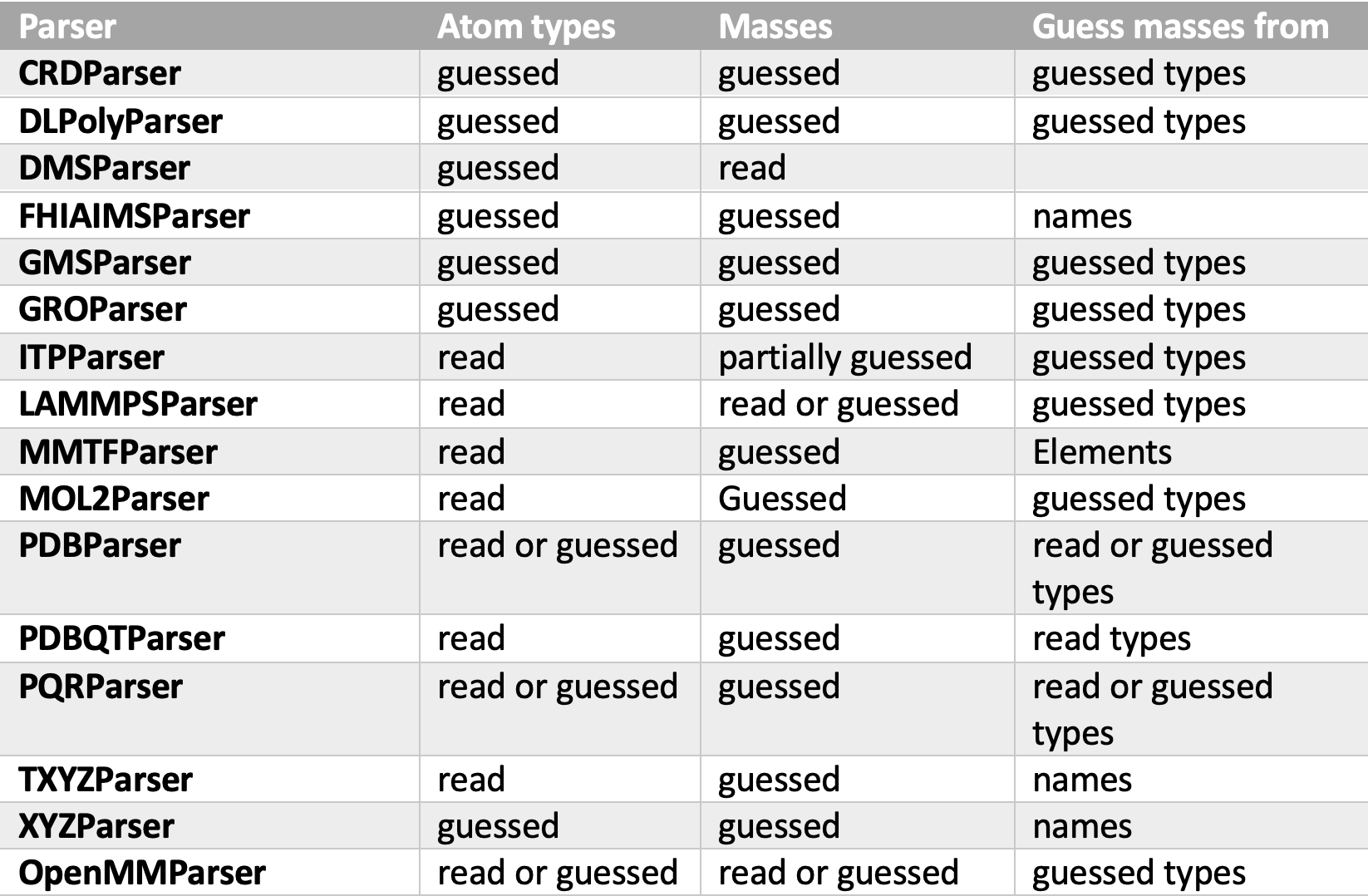
As we see, not all parsers use the same attribute in guessing masses. The DefaultGuesser guesses masses by first looking for the elements attribute and if not available, it looks for the types attribute, this behavior preserves the default behavior of all parsers except the ones that guess masses from names. Parsers that guess masses from types are FHIAIMSParser, TXYZParser, and XYZParser. For both FHIAIMSParser and XYZParser element attributes are provided, and luckily it is just a copy of the names attribute, so the default behavior of these parsers is not affected. For TXYZParser, I added a feature of publishing Elements attribute to its topology output in case all read names are valid elements (merged PR #3836).
- Developing the guess_topologyAttributes API
As described in issue # 3704, the new guesser API will have the tasks of guessing and adding new topology attributes to the Universe. The user only passes the context (eg. “default”, “pdb”, “martini”) and the attributes of interest to be guessed, either through the to_guess or force_guess parameters and the API does the rest. Since I was writing my proposal, I was keen to develop the guesser API with this high level of abstraction and make guessing attributes easy and straightforward to the user without bothering about which method should be called and which attribute(s) is used as a reference in guessing other attributes, so all this work is handled inside the API and the guessers classes. The guess_topologyAttributes() make the following processes:
-
gets the appropriate Guesser class that matches the passed context.
-
checks if the Guesser class support guessing the attributes passed to theto_guess and/or force_guess parameters.
-
check if any attribute passed to the to_guess parameter already exists in the topology attributes of the Universe. If so, warn the user that only empty values will be filled for this attribute, if any exists and in case the user wishes to override all the attribute values, he must pass it to the force_guess parameter instead of the to_guess one.
-
guessing attributes is handled by the guess_attrs method(), which is declared inside the parent guesser class GuesserBase. It manages partial and complete guessing of attributes and calls the appropriate guesser method for each attribute.
-
each attribute guesser method searches for the reference attribute to begin guessing from it, and if not found in the Universe, it calls the guess_topologyAttributes to try guessing this reference attribute.
-
after guessing the attribute, the API adds it to the Universe with the help of add_topologyAttr or _add_topology_objects Universe’s methods
Example of using the guess_topologyAttributes at Universe initiation:
# to guess bonds for a [Universe]:

import MDAnalysis as mda
from MDAnalysisTests.datafiles import two_water_gro

u = mda.Universe(two_water_gro, context='default', to_guess=['bonds'])
Example of using the guess_topologyAttributes directly:
# guess masses and types attribute::

u.guess_TopologyAttributes(context='default', to_guess=['masses', 'types'])
Example of passing empty to_guess list to guess_topologyAttributes so no guessing takes place at universe creation:
# silencing masses and types guessing at universe creation::

import MDAnalysis as mda
from MDAnalysisTests.datafiles import two_water_gro

u = mda.Universe(two_water_gro, to_guess=())
More explanation is found in the user guide here: guess_topologyAttributes, Guessing
The DefaultGuesser class holds the same old guessing methods but with modifying them to be compatible with the new guess_topologyAttrsibutes API. Moreover, I added a new feature to type guessing method so that it now can guess types from masses if names are not available (commit 348f62d)
- Testing the old parser behavior is preserved
The to_guess parameters of the Universe have a default value of ("types", "masses") to maintain the default behavior of the parsers. To make sure of not breaking old behavior, I added three tests in the parser’s base.py module to check three things:
-
types and masses are guessed as expected in all Universe’s created with the parsers after removing guessing from them.
-
The values of the guessed types with the guess_topologyAttributes API are the same as those from the old behavior.
-
The values of the guessed masses with the guess_topologyAttributes API are the same as those from the old behavior.
Once those three tests are passed, then it’s safe to say that we are not breaking the default behavior of the code (commit af84927).
I also discovered a bug in Topology’s methods gussed_attributes() and read_attributes() while working on developing the guesser API and fixed it (merged PR # 3779)
2- Working on PDBGuesser
Currently, I’m working on developing the PDBGuesser issue #3856. The generic guessing methods can’t deal optimally with PDB files, which makes guessing processes slow and not reliable for pdb-generated topologies. So, if we had a PDB-aware guesser, this process could improve significantly, especially that PDB has a huge archive called the chemical component dictionary (CCD), which describes every single residue that exists in the PDB database (its atom names, atom elements, bonds, bond orders, charges, aromaticity, etc.), plus that PDB has a well-formatted structure, that makes it easy to infer topology properties from it. I’m working on developing guesser methods for elements, masses, bonds, and aromaticity.
a. Elements guessing
PDB has a well-defined format for names, from which we can get the atomic symbol easily.
Atom names are found in columns 13-16. The first two characters represent the atom symbol, and if the symbol consists of one character, then the first character is blank. At the third character comes the remoteness indicator code for amino acid residues ['A', 'B', 'G', 'D', 'E', 'Z', 'H']. Then the last character is a branching factor if needed.
The above rules are the standard rules but there are some exceptions to them:
-
If the first character is blank and the second character is not recognized as an atomic symbol, we check if the third character contains “H”, “C”, “N”, “O”, “P” or “S”, then it is considered the atomic symbol.
-
If the first character is a digit, ”, ’, or *, then the second character is the atomic symbol.
-
If the first character in ‘H’ and the residues are a standard amino acid, nucleic acid, or known hetero groups (found in pdb_tables.py), then the atom element is ‘H’.
-
If the first two characters are not recognized as an atomic symbol and the first character is ‘H’, then the element is H.
Based on these rules, I developed the guess_types method for PDBGuesser pr #3866.
b. Masses
Mass guessing is the same as generic mass guessing methods, I just added a more detailed message about how many successful guessings happened and how many failed, in addition to which atom type/element the guesser failed to guess mass to.
PDBGuesser is still under discussion, so some of the current implementations may be updated in the future.
Future work
I’m currently working on the PDBGuesser and plan to implement the MartiniGuesser after the GSoC period. Completing those context-aware guessers is not just important for having more tailored guessers, but also crucial for testing how the new guesser methodology is flexible and can work fine with different types of Guessers classes that will be implemented in the future.
Lessons learned
GSoC was my first software internship, and I feel lucky that I got the chance to participate in such a wonderful program under the MDAnalysis organization, where everyone is supportive and friendly. I have learned about contributing to the open-source community, and the value of being a part of it. I also learned more about software engineering principles and how to better estimate the time and effort needed for your work. Additionally, I learned how to set priorities in developing new features, and the importance of test-driven software development. Finally, I learned how to effectively communicate and represent my work, and the importance of clean code and well-documented steps.
I’m happy with my experience with MDAnalysis and looking forward to increasing my contribution to the library, especially in the guessing and topology parts which I gained lots of experience at.
Acknowledgements
I’d like to thank all my mentors for their effort and valuable lessons they gave to me through the program period, and I’m
specially gratful for @jbarnoud (Jonathan Barnoud) for his endless guidance and patience through every step in the project.
For more information about the details of my journey with GSoC throught the summer you can check my personal blog post Here.
– @aya9aladdin
20 Nov 2022
Motivation
In molecular dynamics simulations, users frequently have to inspect energy-like terms such as potential or kinetic energy, temperature, or pressure. This is so common a task that even small inefficiencies add up. Currently, users have to create intermediate files from their MD simulation’s output files to obtain plot-able data, and this quickly becomes cumbersome when multiple terms are to be inspected. Being able to read in the energy output files directly would make this more convenient.
Therefore, I wanted to add readers for energy-type files (output files containing information on potential and kinetic energy, temperature, pressure, and other such terms) from a number of MD engines to the auxiliary module of MDAnalysis in this project. This would make quality control of MD simulations much more convenient, and allow users to analyse the energy data without the need for switching windows or writing intermediate files directly from within their scripts or jupyter notebooks.
In a first instance, I focussed on a reader for EDR files, which are energy files written by
GROMACS during simulations. EDR files are binary files which follow the XDR protocol. To read these
files, @jbarnoud had previously written the panedr Python package, which was the
foundation of my work this summer.
Adapting Panedr for use in MDAnalysis
The panedr package makes use of the xdrlib Python module to parse EDR files
and return the data in the form of a pandas DataFrame. My GSoC project started out
adapting this package for use in MDAnalysis. In particular, we wanted to avoid making
pandas a dependency in MDAnalyis. This necessitated some refactoring of panedr (PR #33),
which ultimately led to a restructuring of the code into two distinct packages: panedr
and pyedr (PRs #42 and #50). Both packages read EDR files, but one returns the
data as a pandas DataFrame, the other as a dictionary of NumPy arrays. Both also
expose a function to return a dictionary of units of the energy terms found in the file (PR #56).
Example:
import pyedr
file = "path/to/edr/file.edr"
energy_dictionary = pyedr.edr_to_dict(file)
unit_dictionary = pyedr.get_unit_dictionary(file)
EDRReader
With Pyedr available, I started work on the implementation of an EDRReader in MDAnalyis (PR #3749).
Here, I benefited hugely from the existing AuxReader framework.
However, from the outset, it was clear that the auxiliary API would need to be changed to accommodate
the large number of terms found in EDR files.
The XVGReader was built under the assumption that auxiliary files would only ever
contain one time-dependent term, so the XVG files would contain a time value and a data value
per entry. Associating data with a trajectory via the add_auxiliary method thus only
required two arguments: a name under which to store the data in universe.trajectory.ts.aux, and the file from which to read it.
This is not suitable for EDR files, as they can contain dozens of terms per time point,
only a few of which might be relevant for a given analysis. Therefore, the auxiliary API had to be changed as follows:
While the XVGReader still works as previously, the new base class for adding auxiliary data assumes a dictionary to be passed. The dictionary maps the name to be used in MDAnalysis to the names read from the EDR file. This is shown in the following minimal working example:
import MDAnalysis as mda
from MDAnalysisTests.datafiles import AUX_EDR, AUX_EDR_TPR, AUX_EDR_XTC
term_dict = {"temp": "Temperature", "epot": "Potential"}
aux = mda.auxiliary.EDR.EDRReader(AUX_EDR)
u = mda.Universe(AUX_EDR_TPR, AUX_EDR_XTC)
u.trajectory.add_auxiliary(term_dict, aux)
Aside from this API change, the EDRReader can do everything the XVGReader can. In addition to that, it
has some new functionality.
- Because EDR files can become reasonably large, a memory warning will be issued when more than a gigabyte of storage is used by the auxiliary data. This default value of 1 GB can be changed by passing a value as
memory_limit when creating the EDRReader object.
- EDR files store data of a large number of different quantities, so it is important to know their units as well. The EDRReader therefore has a
unit_dict attribute that contains this information. By default, units found in the EDR file will be converted to MDAnalysis base units on reading. This can be disabled by setting convert_units to False on creation of the reader.
- In addition to associating data with trajectories, the EDRReader can also return the NumPy arrays of selected data, which is useful for plotting, for example. This is done via the EDRReader’s
get_data method.
Additionally, the new auxiliary readers allow the selection of frames based on the
values of the auxiliary data. For example, it is possible to select only frames
with a potential energy below a certain threshold as follows:
u = mda.Universe(AUX_EDR_TPR, AUX_EDR_XTC)
term_dict = {"epot": "Potential"}
u.trajectory.add_auxiliary(term_dict, aux)
selected_frames = np.array([ts.frame for ts in u.trajectory if ts.aux.epot < -524600])
Having selected these frames, it is possible to analyse only this subset of a trajectory:
protein = u.select_atoms("protein")
for ts in u.trajectory[selected_frames]:
    do_analysis(protein)
More details on the EDRReader’s functionality can be found in the MDAnalysis User Guide.
Outlook
Through this project, the AuxReader framework was expanded, and handling of EDR
files was made more convenient with pyedr and EDRReaders. I am continually making
improvements to these contributions, and will include an auxiliary reader for
NumPy arrays in the future. This NumPyReader will be very useful, because many
analysis methods in MDAnalysis return their results in the form of NumPy arrays.
Having the option of associating these results with trajectories will facilitate
further analyses, for example allowing the slicing of trajectories by RMSD to a reference
structure.
In general, the changes made to the auxiliary API should make it easier for
additional AuxReaders to be developed. Being able to easily associate any number of terms
to each time step is helpful for general readers (for example for parsing CSV data)
and for more specific readers (for parsing energy files generated by other MD engines, for example Amber or NAMD).
With the actual handling of the data already taken care of, the challenge in the implementation here would
lie in the correct parsing of the plain text files, and in proper testing and future proofing.
Lessons learned
Participating in the Summer of Code was a great opportunity for me. I learned a lot, from small things like individual code patterns to larger points concerning overall best practices, the value of test-driven development, and package management. This is thanks in large part
to the mentorship and advice I have received from @hmacdope, @ialibay, @orbeckst, and @fiona-naughton.
Thanks very much to you all, and to @jbarnoud.
– @bfedder