02 Sep 2021
Motivation
My research seeks to discover new materials for battery electrolytes. In particular, I use molecular dynamics and ab initio methods to computationally probe new electrolyte compositions. In my work, a core challenge is scaling up. A molecular dynamics trajectory is a rich and complex data structure, thorough analysis requires interactive visualization and data labeling. Automating this sort of interactive analysis is difficult, but to scale up to hundreds or thousands of electrolytes, it needs to be done.
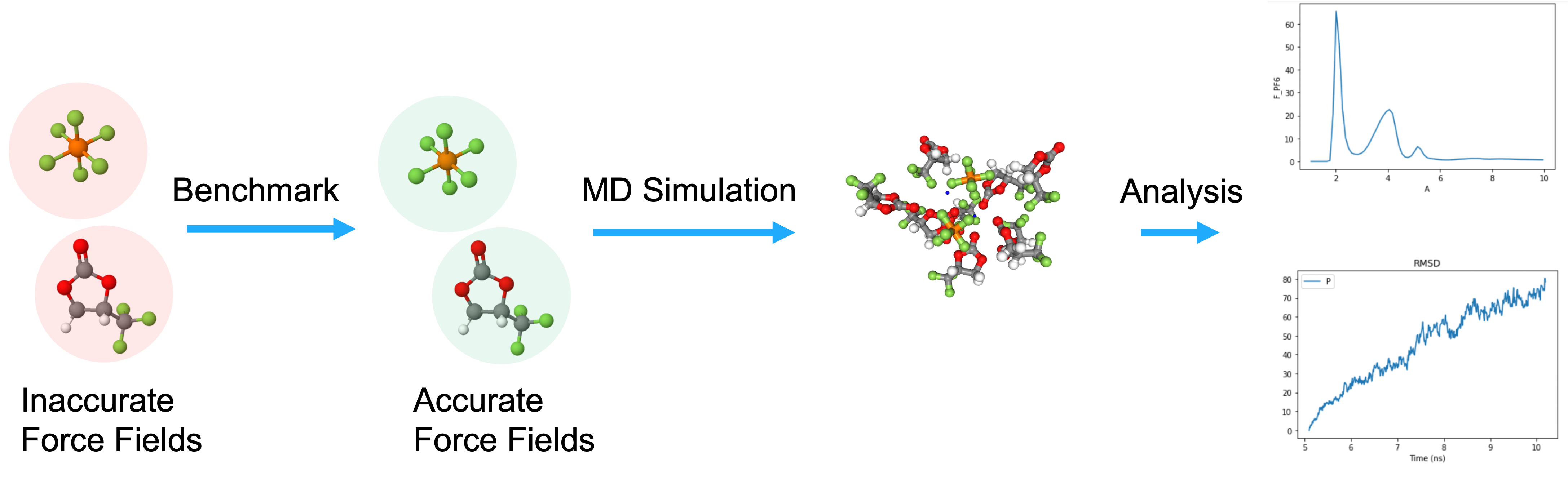
I applied for Google Summer of Code because I felt that MDAnalysis was the best available tool for the automated analysis of MD trajectories. My aim was to build an abstraction around solvation that would make writing automated analysis methods much easier. Over the past few months, I’ve done that. I am now working to refine the API and implement new methods to extract more information from MD simulations. In time, this will fit into a broader workflow that will enable the autonomous exploration of novel electrolytes.
Retrospective
At the outset of my GSoC project, I hoped to create a package with:
- Functions for selecting the solvation shells of ions.
- Automated analysis of ion coordination environment.
- Documentation, testing, and well-written code.
After 10 weeks of working with the MDAnalysis team, the solvation_analysis package vastly exceeds that original intent. There is a robust and simple API, the functionality generalizes to non-ionic systems, solvation distances are automatically identified, and it’s really fast. Further, I’ve learned a huge amount about software development, the package release cycle, and the world of open-source.
In this post, I will summarize my contributions to solvation_analysis and several features of the package.
My Summer in Pull Requests
Template for a snazzy package
PR #7 and #20
My summer began with a duo of pull requests. PRs #7 and #20 filled out the template generated by the MolSSI cookiecutter, creating a fashionable scaffold that my code could fit into. In essence, the PRs set up the trappings of a real package, assuring users (and myself) of a certain core competence in the development.
Testing, testing, one-two-three
PR #6, #16, and #17
Robust testing is part of a finished package. PR #6 introduced the initial code base and some rudimentary testing. In PR #16, I started using pytest, which made writing and using tests much easier. Finally, PR #17 integrated testing with GitHub CI, finalizing a critical component of my development workflow.
Cutting off radial distribution functions
PR #25
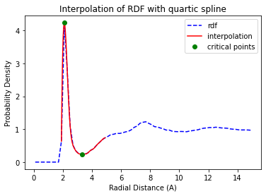
PR #25 was a science challenge in addition to a software challenge. I needed to robustly identify the first minima of noisy RDF data so I could automate the solvation analysis. My approach was to perform a polynomial interpolation of the RDF and then take the 2nd-derivative to find the minima. This worked well for smooth RDFs but failed for RDFs with noise. As a quick fix, I added in several heuristics to get the solvation distances identified on my noisy test data. For now, the RDF parser works reasonably well for smooth data and warns users when it fails. An interpolation of an RDF is shown below.
Analysis: the mega-PR
PR #29
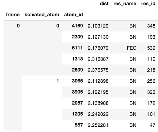
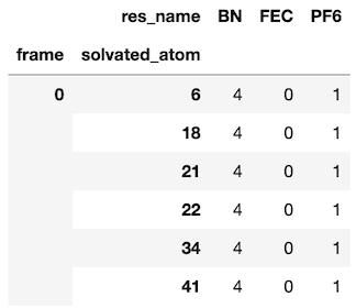
PR #29 is responsible for the majority of functionality in solvation_analysis. It implemented the Solution class and all of the analysis functions, reaching 250 comments from myself and my mentors. Much of the discourse focused on iterating through API designs, which eventually led to a very clean Solution-centered package. The underlying data structure uses the ‘tidy data’ concept, implementing a tidy Pandas.DataFrame that allows analyses to be easily vectorized. As shown below, the DataFrame is indexed by step in the analysis (frame), the solvated_atom from the solute, and the solvent atoms atom_id. This solution provides a unique identifier for each atom participating in solvation.
In pursuit of user number one
PR #36
PR #36 introduced a tutorial to walk users through the basic functionality of solvation_analysis and how to respond to common errors. If you are interested in using the solvation_analysis, this is definitely the best place to start!
Release and versioning
PR #37
I was shocked by how easy it is to release a package to PyPI. For this PR, I learned to use versioneer and twine for Python release management. With just a few terminal commands and file edits, I was able to set up a functioning release management system and put out version 0.1.1.
Solvation Analysis in Practice
Since solvation analysis is up on PyPI, it can be installed with a pip!
>>> pip install solvation_analysis
As in any MDAnalysis workflow, we start by importing the package and instantiating an MDAnalysis Universe.
# imports
import MDAnalysis as mda

# define paths to data
data = "../solvation_analysis/tests/data/bn_fec.data"
traj = "../solvation_analysis/tests/data/bn_fec_short_unwrap.dcd"

# instantiate Universe
u = mda.Universe(data, traj)
Next, we need to define the solute and solvents of interest. The example system is a LiPF6 electrolyte with BN and FEC as solvents. Here, we treat the Li+ ion as the solute and all other molecules as solvents.
# define solute AtomGroup
li_atoms = u.atoms.select_atoms("type 22")

# define solvent AtomGroups
PF6 = u.atoms.select_atoms("byres type 21")
BN = u.atoms.select_atoms("byres type 5")
FEC = u.atoms.select_atoms("byres type 19")
Once we have the universe, solute, and solvents defined, it is quite simple to instantiate and run a solution! Solution, like all MDA analysis classes, subclasses the AnalysisBase class and requires a Solution.run() call to initiate the analysis.
# instantiate solution
from solvation_analysis.solution import Solution

solution = Solution(li_atoms, {'PF6': PF6, 'BN': BN, 'FEC': FEC})

solution.run()
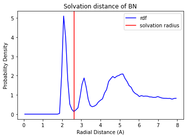
Over the course of a few seconds, the solvation radii and the solvation shell of each ion are automatically identified and stored in a pandas.DataFrame (as described above). We can then examine how well the solvation radii were characterized by calling solution.plot_solvation_radius('<<solvent name>>'). For example,
# we just need this to display our plot
import matplotlib.pyplot as plt

solution.plot_solvation_radius('BN')
plt.show()
Now that we have a completed solution, we can easily print the ion pairing, coordination numbers, and solvation radii.
>>> solution.pairing.pairing_dict
{'BN': 1.0, 'FEC': 0.21, 'PF6': 0.12}
>>> solution.coordination.cn_dict
{'BN': 4.33, 'FEC': 0.25, 'PF6': 0.12}
>>> solution.radii
{'PF6': 2.60, 'BN': 2.61, 'FEC': 2.43}
We can see that the Li+ ions coordinate most strongly with BN. The pairing shows that 100% of Li+ are coordinated with BN and on average there are 4.33 BN coordinated to each Li+. Similar information is available for FEC and PF6.
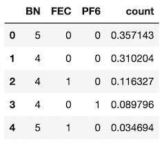
We can also use solvation_analysis and a simple Pandas operation to identify the most common solvation shell compositions and find examples of them for visualization. Below, we are using the speciation class to find the most common compositions of solvation shells and then filtering out all shells with a frequency less than 2%.
solution.speciation.speciation_percent.query("count > 0.02")
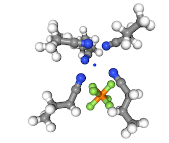
We can pick out a specific examples of that shell for visualization. First we find all shells with a given composition.
# find all shells matching the given dictionary
solution.speciation.find_shells({'BN': 4, 'FEC': 0, 'PF6': 1})
Then we select the solvation shell and use our favorite visualization package to view it!
# get the shell atoms
atoms = solution.solvation_shell(6, 0)

# visualization is not covered here. I suggest nglview!
visualize(atoms)
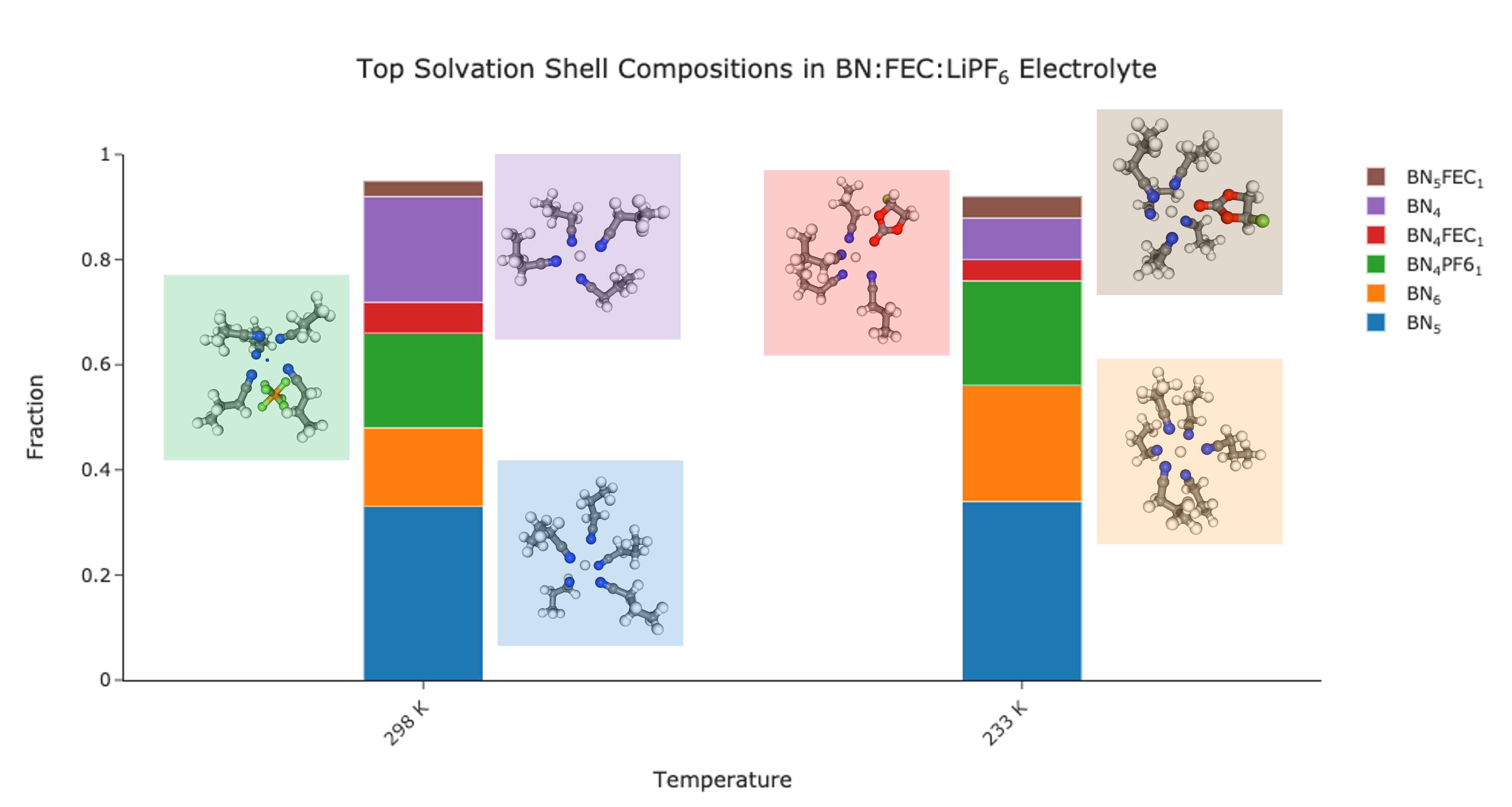
Using that approach, you can find all the common solvation shells and generate visualizations for each. For example, see this speciation plot of the BN:FEC system from the example. I’ve plotted the fraction of each solvation shell at two temperatures and then visualized examples of those shells in the margin.
Together, the tools described above are a powerful and convenient workflow for analyzing the solvation structure of a liquid. Several analyses are pre-implemented and the core solvation data structure makes it easy to create new methods. I sincerely hope that it is useful to the community!
The Future
PR #39 and #40
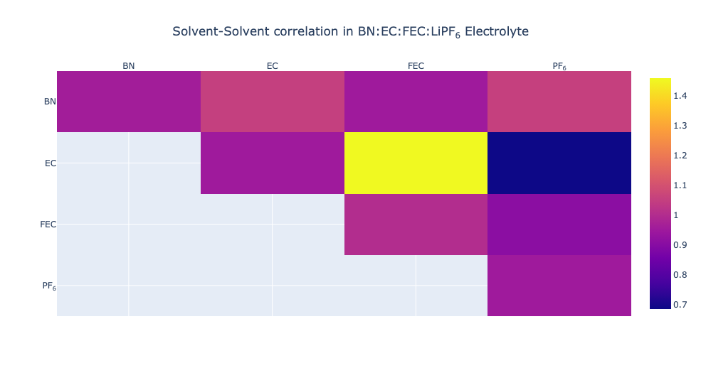
While GSoC has ended, development of solvation_analysis has not. PR #39 adds solvent correlation analysis, statistics on uncoordinated solvents, and a new Valency class. PR #40 introduces a tutorial on interactive visualization. These are all features I am excited for and look forward to developing. As a teaser, I’ll include a correlation plot below:
Acknowledgements
As a whole, the MDAnalysis was incredibly welcoming and helpful. I am genuinly inspired by the dedication and competence of the core developers of the package. I am especially grateful for the help of @hmacdope (Hugo), @richardjgowers (Richard), and @IAlibay (Irfan), who were excellent mentors and are generally talented and kind individuals.
I am also thankful for Google’s generous support of open source software.
It has been an amazing ride 🎢
– @orioncohen
02 Sep 2021
The main goal of my GSoC project
was to develop a tool to calculate membrane curvature
from MD simulations using MDAnalysis. We
aimed to have the following features in the membrane curvature analysis tool:
- Surfaces derived from an
AtomGroup of reference.
- Calculation of mean and Gaussian curvature.
- Multiframe and averaged-over-frames analysis.
- Plug-and-play with visualization libraries to obtain 2D curvature profiles.
- Data visualization made easy.
Why Membrane Curvature?
In the wide range of tools that are available to analyze Molecular Dynamics (MD)
simulations, user-friendly, actively-maintained, and well-documented tools to
calculate membrane curvature are still difficult to find. I was motivated to
share a tool to calculate membrane curvature that I initially developed as part
of my PhD at the Biocomputing Group.
Membrane curvature is a phenomenon that can be investigated via MD simulations, and
I had an interest to share this tool with the wider MD community.
Contributions
Keeping in mind the goals and motivations behind my GSoC project,
I would like to hightlight three areas of contributions that were key to the
MembraneCurvature MDAnalysis tool: Core functions,
AnalysisBase, and Documentation.
Core functions (#9, #34, #40, #44)
The initial version of the code contained functions to map elements from
the AtomGroup of reference into a grid of dimensions defined by the simulation
box. The initial version also included the functions to calculate mean and Gaussian curvature.
After refactoring, the core functions of MembraneCurvature were cleaned
and tuned up. In summary, our core functions can be split into two groups:
-
Surface :
derive_surface(), get_z_surface(), normalize_grid().
-
Curvature :
mean_curvature(), gaussian_curvature().
These functions are our bricks to build the MembraneCurvature AnalysisBase.
Analysis Base (#43, #48)
The analysis in MembraneCurvature used the
MDAnalysis AnalysisBase
building block, from where we obtained the basic structure to run multilframe analysis.
In the MembraneCurvature subclass of AnalysisBase,
we define the initial arrays for surface, mean, and Gaussian curvature in the
_prepare() method. In _single_frame(), AnalysisBase runs the
membrane curvature analysis in every frame, and populates the arrays previously
defined in _prepare(). In _conclude, we compute the average over frames for
the surface and curvature arrays (#43).
The derived surface and calculated arrays of mean and Gaussian curvature values
are stored in the results attribute. This makes AnalysisBase the most
fundamental part of the MembraneCurvature analysis, allowing us to perform
multiframe and average-over-frame curvature analysis.
We also added coordinate wrapping
to our Analysis base, which enables users to run MembraneCurvature with all
atoms in the primary unit cell (#48). Having an option to wrap coordinates is
particularly useful when we want to calculate curvature with elements in the
AtomGroup that may fall outside the boundaries of the grid.
With #48, we also achieved a significant milestone: reaching 100% code
coverage
in MembraneCurvature! 100% coverage means that every line of
code included was executed by pytest, the test suite used by MDAnalysis, to check that the code works as it
should.
One of the strongest motivations to contribute an MDAnalysis
curvature tool was to provide a well-documented package
to analyze membrane curvature from MD simulations.
The membrane curvature tool includes solid documentation that can be found in
the following pages:
We included two different tutorials: One where we use Membrane Curvature to
derive surfaces and calculate curvature of a membrane-only system. A second tutorial to calculate curvature in a membrane-protein system is currently under development (#69).
How can I use it?
Membrane-curvature uses MDAnalysis under the hood. We can install
Membrane-curvature via pip:
pip install membrane-curvature
Here you can find more installation instructions.
Running MembraneCurvature
MembraneCurvature was designed to be user friendly. No counterintuitive
commands, and no long lines of code. With MembraneCurvature you can calculate
curvature in just a few lines! The snippet below illustrates how easy it
gets to extract mean and Gaussian curvature from MD simulations using MembraneCurvature:
import MDAnalysis as mda
from membrane_curvature.base import MembraneCurvature
from membrane_curvature.tests.datafiles import (MEMB_GRO,
                                                MEMB_XTC)

u = mda.Universe(MEMB_GRO, MEMB_XTC)

mc_upper = MembraneCurvature(u,
                             select="resid 103-1023 and name PO4",
                             n_x_bins=12,
                             n_y_bins=12).run()

mc_lower = MembraneCurvature(u,
                             select='resid 1024-2046 and name PO4',
                             n_x_bins=12,
                             n_y_bins=12).run()
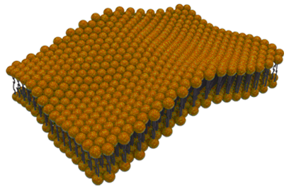
In the example above, we use two files included in the MembraneCurvature tests:
MEMB_GRO and XTC_GRO, which comprises a membrane of lipid composition
POPC:POPE:CHOL, in a
5:4:1 ratio:
We use the selection "resid 103-1023 and name PO4" as an
AtomGroup of reference to derive the surface associated to the upper leaflet.
Similarly, we derive the surface from the lower leaflet with the AtomGroup
defined by the selection "resid 1024-2046 and name PO4" . In this example,
PO4 is the name of the phospholipid head groups.
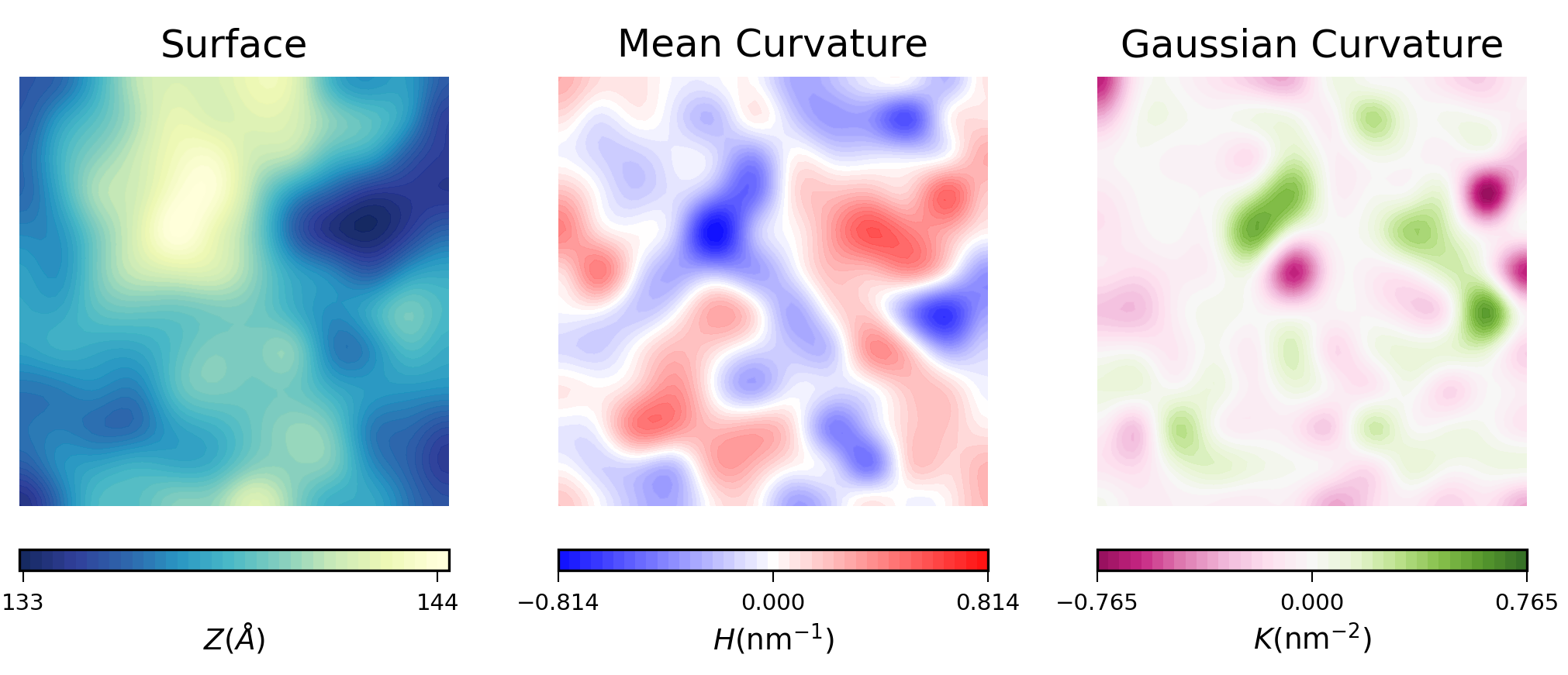
After running MembraneCurvature, the calculated values of the derived surface
(H), and Gaussian curvature (K) are stored in the _results() attribute. We
can easily extract the average results with:
# surface
surf_upper = mc_upper.results.average_z_surface
surf_lower = mc_lower.results.average_z_surface

# mean curvature
mean_upper = mc_upper.results.average_mean
mean_lower = mc_lower.results.average_mean

# Gaussian curvature
gauss_upper = mc_upper.results.average_gaussian
gauss_lower = mc_lower.results.average_gaussian
Plots
To visualize the results from MembraneCurvature.run(), we can use contourf or imshow from Matplotlib.
For example, here is the plot of the averaged results for the upper leaflet using contours:
In biological membranes of higher complexity, lipid composition between leaflets
is commonly assymetric. With the results obtained from
MembraneCurvature, direct comparison between leaflets can be easily performed. The following snippet generates a
side-by-side plot of the mean curvature results for each leaflet with its respective color bar:
import matplotlib.pyplot as plt
from scipy import ndimage
import numpy as np

results = [mean_lower, mean_upper]
leaflets = ["Lower", "Upper"]

fig, [ax1, ax2] = plt.subplots(ncols=2, figsize=(4,3.5))
max_ = max([np.max(abs(h)) for h in results])

for ax, rs, lf in zip((ax1, ax2), results, leaflets):
    rs = ndimage.zoom(rs, 4, mode='wrap', order=1)
    levs = np.linspace(-max_, max_, 40)
    im = ax.contourf(rs, cmap='bwr',
                     origin='lower', levels=levs,
                     vmin=-max_, vmax=max_)

    ax.set_aspect('equal')
    ax.set_title('{} Leaflet'.format(lf), fontsize=6)
    ax.axis('off')

cbar = plt.colorbar(im, ticks=[-max_, 0, max_],
                    orientation='vertical',
                    ax=[ax1, ax2], shrink=0.4,
                    aspect=10, pad=0.05)
cbar.ax.tick_params(labelsize=4, width=0.5)
cbar.set_label('H (nm$^{-1}$)', fontsize=6, labelpad=2)
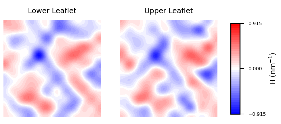
Mean curvature plots provide information about the “inverted shape” of the surface,
which in this example is derived from phospholipids headgroups in each leaflet.
Positive mean curvature indicates valleys (red coloured), negative mean curvature is associated
with peaks (blue coloured). Regions where H=0 indicates a flat region (white coloured). In the
example considered here, the contour plot of mean curvature shows:
-
Coupling between leaflets. Regions of positive curvature (red coloured) in the
lower leaflet match those in the upper leaflet. The same is observed for
regions of negative curvature (blue coloured).
-
A central region of negative curvature. For both upper and lower leaflets,
there is a central region of negative mean curvature (blue coloured) along the
y axis, while regions of positive curvature (red coloured) are localized in
the bulk of the membrane, in particular bottom left and upper right regions.
In progress
Currently, we are working on implementing interpolation as an option for the
user #52.
In some situations, when selecting a very high number of bins in the grid, or
when having regions of the grid with low sampling we may find regions of undefined values.
For example, think of a membrane-protein system, where the bins occupied by the protein won’t be
populated by lipids, and therefore, will have a region of undefined values in
the grid. Such undefined values spread in the array during the calculation of
curvature, which may result in meaningless output.
By adding an optional interpolation, we will be able to patch up undefined values
in bins inside the embedded element (i.e. protein). With this improvement, calculation
of membrane curvature won’t be hamstrung by the presence of undefined values in the grid.
What’s next?
There is always room for improvement, and MembraneCurvature is not an exception.
One of the main limitations of the current version of MembraneCurvature is the
inability to calculate curvature in systems like vesicles, capsids, or micelles.
This would definitely be a nice improvement for a future release of
MembraneCurvature!
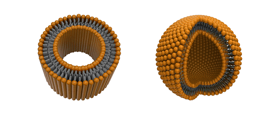
We acknowledge that scientific research would benefit from a
tool to calculate membrane curvature in these types of systems, so we are
considering possible approaches to include more topologies in MembraneCurvature!
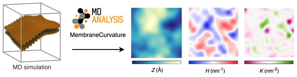
Summary
MembraneCurvature is a well-documented and easy-to-use tool to derive 2D maps of mean and Gaussian
curvature from Molecular Dynamics (MD) simulations. Since it uses the
MDAnalysis AnalysisBase
building block, MembraneCurvature enable users to perform multiframe and
average-over-frames curvature analyses.
From MD simulations to 2D curvature profiles in only a few lines of code!
Acknowledgments
Participating in GSoC with MDAnalysis has been a unique experience. I had the
opportunity to learn best practices in software development mentored by a group
of incredibly talented people:
I also would like to thank @richardjgowers (Richard) and @tylerjereddy (Tyler)
from the MDA community, who participated in our discussions and provided
valuable insights.
Thanks for all your valuable lessons.
MembraneCurvature has launched! 🚀
— @ojeda-e
31 Aug 2021
MDAnalysis is excited to announce that we have been awarded an Essential Open Source Software for Science (EOSS) grant by the Chan Zuckerberg Initiative for our proposal “MDAnalysis: Faster, extensible molecular analysis for reproducible science”.
Over the next two years, this award will fund work on two major aims that will improve MDAnalysis for our users and make it easier for scientists to contribute code, with a view towards increasing code reuse, interoperability, and reproducibility:
As MDAnalysis has now become a mature library with a stable API, we want to focus on improving the performance of core library components by rewriting essential code in Cython. This will enable us to handle the increasingly large and complex datasets generated to solve the biomedical challenges of tomorrow.
(2) Launching the “MDAKits” ecosystem
We will launch the MDAnalysis Toolkits (“MDAKit”) ecosystem. Inspired by SciPy’s SciKits, an MDAKit will contain code based on MDAnalysis that solves specific scientific problems. An MDAKit can be written by anyone and hosted anywhere. In order to streamline the process we will provide a cookiecutter-based template repository. MDAKits will have a well-defined API, have documentation, will be registered with MDAnalysis, and will be continuously tested for compatibility with the current version of MDAnalysis. As part of the registration process, code will be reviewed by MDAnalysis developers and we will encourage the scientific publication of the package, e.g., in the Journal of Open Source Software. We will also refactor a number of analysis modules as separate MDAKits. Overall, the introduction of MDAKits will enable the rapid development and dissemination of new components and tools that can be released independently of the main package. We will soon describe the details of MDAKits in a white paper and seek a discussion with the wider community. Ultimately, MDAKits should help address two long-standing challenges in the biomolecular simulation community: effort duplication and reproducibility.
Along the same lines, we will focus on software interoperability with other packages by expanding our converters framework.
By validating, maintaining and publicizing new code through a common process, we encourage scientists to reuse and extend existing packages rather than re-creating their own ones. We hope that this combined approach will improve consistency, transparency, and accessibility in methods used across scientific studies.
This project will be led by Irfan Alibay, Lily Wang, Fiona Naughton, Richard Gowers, and Oliver Beckstein.
About MDAnalysis
The MDAnalysis package is one of the most widely used Python-based libraries for the analysis and manipulation of molecular simulations. The objective of MDAnalysis is to provide simple, flexible, and efficient means of handling molecular structure data from simulations and experiments and support research in biophysics, biochemistry, materials science and beyond.
MDAnalysis is a fiscally-sponsored project of NumFOCUS, a nonprofit dedicated to supporting the open source scientific computing community.